Prefill, decode and KV cache: choosing hardware for an LLM (2026)
An LLM does not stress hardware the same way when it reads your request as when it writes its answer. Understanding the two phases, and the role of memory bandwidth, is what lets you choose the right card and the right architecture, from a workstation to a rack.

The two phases of an LLM: prefill and decode
A generation unfolds in two phases with opposite hardware demands. Prefill processes your entire request in one pass: system prompt, context and question. These are large matrix-by-matrix multiplications, perfectly parallel, that saturate the card's compute. This phase is compute-bound and sets the delay before the first token. A high-power GPU, with native FP4 or FP8 support, shortens it.
Decode writes the response one token at a time. Each token depends on the previous ones; these are matrix-by-vector operations that do little compute but reread a large amount of data. This phase is bound by memory bandwidth and sets the generation speed, the time between two tokens. Compute intensity drops to a few dozen operations per byte here, and GPU utilisation often falls below half. The resulting rule is simple: prefill demands FLOPS, decode demands bandwidth.
Decode is bound by memory bandwidth
Since generation rereads all the model's weights at every token, speed depends directly on how fast the card reads its memory. This is the decisive factor, and it varies by a factor of thirty depending on the solution.
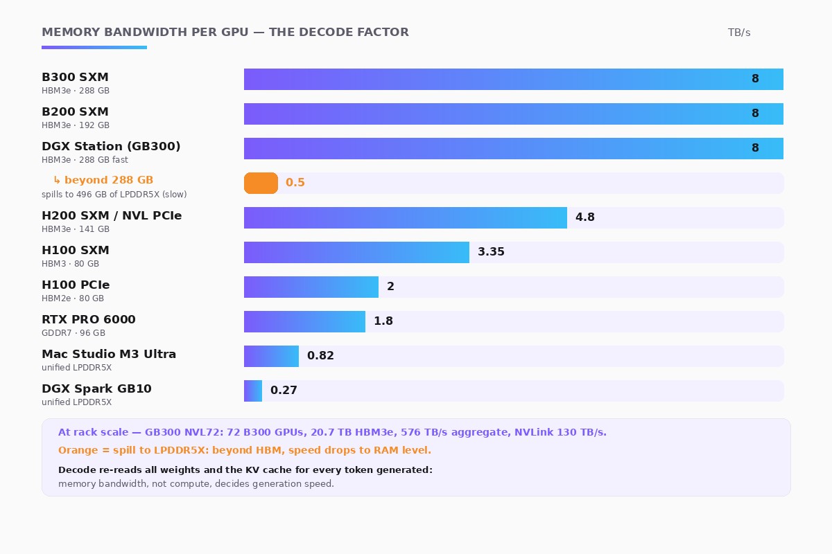
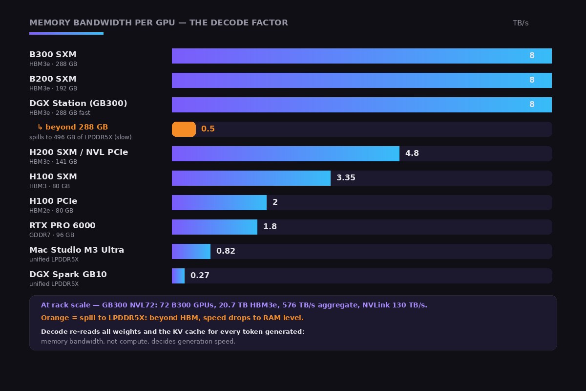
One example puts a figure on the gap. On the same compact model, the RTX PRO 6000 server generates around 215 tokens per second where a DGX Spark tops out around 50, four times slower, even though both load the model with ease. On a seventy-billion-parameter model, a single Spark drops to just a few tokens per second in generation: its 128 GB of memory loads the model, but its 273 GB/s of bandwidth cannot serve it fast. At the other end of the scale, an H200, B200 or B300 rack targets maximum throughput for long context and large-scale serving, and a GB300 NVL72 rack pushes coherent memory to 20.7 TB across seventy-two cards.
The DGX Station illustrates a trap, flagged in orange on the diagram. Its 288 GB of HBM3e serve at 8 TB/s, but the machine adds 496 GB of much slower LPDDR5X. As long as the model and the KV cache fit within the 288 GB of HBM, generation is fast. As soon as they spill over into LPDDR5X, that portion is read at RAM speed, a few hundred gigabytes per second, and decode slows down sharply on the overflowed part. The large capacity is there to load very large models, not to serve all of them at full speed.
The KV cache, what weighs down decode
To avoid recomputing everything at every token, the model stores the keys and values of attention in a KV cache. This cache grows with context length, the number of concurrent requests and the number of layers. Over long responses and several users, it can exceed the size of the model itself. Since it is reread at every token, it worsens the decode bottleneck and takes up video memory.
Three levers keep it in check: grouping attention heads, or GQA, which reduces the number of keys and values to store; KV cache quantization, which compresses it; and a controlled context length. This is also why very long context first demands memory bandwidth, before any other optimisation.
What has to fit on a card
"The model fits on the card" is not limited to the weights. Four items share video memory, and the last one is variable: the model's weights, the embedding model and the reranker in a RAG pipeline, and the KV cache, which grows with context and the number of requests.
Take a concrete example: Qwen3.6 35B A3B in NVFP4, 256K-token context, on a 96 GB RTX PRO 6000. The A3B label means 3 billion parameters are active per token, but all 35 billion reside in memory, since a mixture-of-experts model loads all of its experts.
| Item | Size (order of magnitude) |
|---|---|
| Qwen3.6 35B A3B weights, NVFP4 (4-bit) | ~18 GB (all 35 B reside) |
| Embedding model, ~4 B in FP8 | ~4 GB |
| Reranker, ~2 B in FP8 | ~2 GB |
| Framework and activations | ~4 GB |
| Fixed subtotal | ~28 GB |
| KV cache for 256K tokens, in FP16 | ~24 GB |
| KV cache for 256K tokens, in FP8 | ~12 GB |
The KV cache is the item that varies. Its size per token equals twice the number of layers, times the number of KV heads, times the head dimension. For an architecture of this type, on the order of forty-eight layers, four KV heads under GQA and a dimension of 128, that comes to roughly 96 KB per token in FP16, so ~24 GB for 256K tokens; half that in FP8 (~12 GB), half again at 4-bit (~6 GB). A 256K-token request with an FP8 KV cache therefore needs roughly 28 + 12 = 40 GB, which fits comfortably on a 96 GB card.
How much context fits, then? After the fixed subtotal (~28 GB), around 68 GB remain for the KV cache. In FP16, at 96 KB per token, that takes a single request to nearly 700,000 tokens; in FP8, beyond a million. In practice, this budget is shared across concurrent requests: at 256K tokens per request with an FP8 KV cache, the card serves around five requests in parallel. Lowering KV cache precision, or enabling GQA, therefore buys context or concurrency directly. Co-locating embedding, reranker and LLM on a single card is the typical pattern for a small sovereign RAG platform; beyond that scale, one card is dedicated to inference and another to the retrieval models.
The interconnect: when several cards must talk to each other
As soon as a model is split across several cards in tensor parallelism, every layer triggers an all-reduce that synchronises the cards, so at every token. The speed of this link then becomes the bottleneck. The orders of magnitude leave no room for doubt.
| Solution | Multi-GPU interconnect | Note (with or without NVLink) |
|---|---|---|
| GB300 NVL72 (rack) | NVLink 5 and NVSwitch, 130 TB/s across the domain | 72 B300 GPUs seen as one, 20.7 TB of coherent memory |
| B300 and B200 SXM | NVLink 5, 1.8 TB/s per card, full mesh | Near-linear tensor parallelism across eight cards |
| H200 SXM and H100 SXM | NVLink 4 and NVSwitch, 900 GB/s per card | Full mesh across eight cards, with NVLink |
| H200 NVL (PCIe) | NVLink bridge up to four cards, 900 GB/s; otherwise PCIe | Same memory bandwidth as the SXM, 4.8 TB/s |
| H100 PCIe | NVLink bridge in pairs, 600 GB/s; otherwise PCIe | Slower memory than the SXM, 2.0 versus 3.35 TB/s |
| Any single PCIe card, no bridge | PCIe Gen5 x16, ~128 GB/s | Seven times slower than NVLink 4, without NVLink |
| DGX Station (GB300) | Internal NVLink-C2C, 900 GB/s between CPU and GPU | Single-GPU workstation, 784 GB of coherent memory |
| DGX Spark cluster (ConnectX-7 RoCE) | 200 Gb/s, i.e. ~25 GB/s | Network link between machines, no switch |
On PCIe, the tensor-parallelism all-reduce drops scaling efficiency to around 0.7, and can consume a third of compute time across eight cards. NVLink, by contrast, keeps this exchange negligible.
One card, or several? PCIe, NVLink, SXM
The right choice follows a clear logic.
- A single card. No interconnect bottleneck. This is the best option when the model fits: the RTX PRO 6000 and its 96 GB then dominates on performance per cost, ahead even of an H100 on single-card throughput.
- Two to eight PCIe cards, without NVLink. Tensor parallelism suffers from the all-reduce. It is better to split the model in a pipeline, which only exchanges once per token, or to run independent replicas to serve several users. PCIe is enough for compact models and large request batches.
- SXM cards with NVLink and NVSwitch. Tensor parallelism scales almost linearly. But in inference, this mesh often goes unused: you pay a third to half more, and double the power draw, for capacity that is mostly useful for training. To serve a model, PCIe is the economical choice, except for very large dense models split at low latency.
Modern engines handle this trade-off: vLLM detects the topology at startup and switches to the all-reduce optimised for NVLink when cards are bridged, otherwise it falls back to PCIe.
Stacking DGX Sparks: capacity, not speed
Linking two DGX Sparks through their ConnectX-7 port pools 256 GB of memory and makes it possible to load a four-hundred-and-five-billion-parameter model in FP4, impossible on a single machine. But the 200 Gb/s link remains slow compared with internal memory. In low-latency serving, NVIDIA states a per-token time that roughly tracks the number of machines. In batch mode, the pipeline clearly outperforms tensor parallelism over this network link. The message fits in one sentence: a Spark cluster unlocks models too large for a single machine, it does not speed up a model that already fits.
How to choose: sizing rules
- The model fits on one card: single GPU, the simplest and best cost per token.
- Latency priority on a very large model: SXM and NVLink, tensor parallelism within the machine.
- Multi-user throughput priority: single-GPU replicas or pipeline, PCIe is enough.
- Very long context, large KV cache: target memory bandwidth, H200 or B200, with GQA and cache quantization.
- Maximum capacity under budget or noise constraints: unified memory, Mac Studio or DGX Spark, capacity comes first, not throughput.
- Several machines: tensor parallelism within the machine via NVLink, pipeline between machines over the network.
Sizing therefore depends on the model, the context length and the number of users, not on one universal king card. Price ranges by tier are covered in our AI server pricing guide, and model choice in our open-source LLM comparison. QDNA integrates this hardware and operates it for you, from a workstation to a rack.
Frequently asked questions
Why does my local LLM generate slowly despite a large GPU?
Generation, or decode, is limited by memory bandwidth, not by compute power. For every token, the card rereads all the weights and the KV cache. A card with large capacity but low bandwidth, such as the DGX Spark at 273 GB/s, can load a large model but generates it slowly.
Do you need NVLink for LLM inference?
Rarely. NVLink matters when a model is split across several cards in tensor parallelism, where an all-reduce synchronises the cards at every token. For everyday inference, PCIe is enough, and NVLink mainly benefits multi-GPU training. For very large models split across cards at low latency, it becomes useful again.
SXM or PCIe to serve an LLM?
PCIe is more cost-effective and sufficient for most inference workloads, since the NVLink mesh on SXM cards often goes unused during generation. SXM is justified for multi-GPU training, where the all-reduce across eight cards requires the NVSwitch's 900 GB/s.
Is the DGX Spark fast for an LLM?
The DGX Spark offers 128 GB of unified memory but only 273 GB/s of bandwidth. It excels at prototyping and with compact models, but generates large dense models slowly. Linking two Sparks unlocks capacity, up to Llama 405B in FP4, not per-token speed.
How do you reduce the size of the KV cache?
Three levers: grouping attention heads, or GQA, which reduces the number of keys and values to store; KV cache quantization, which compresses these activations; and a controlled context length, since the cache grows with conversation length and the number of concurrent requests.
Let's size your hardware to your real usage
A call to scope the card, the architecture and the runtime against your models, your context length and your number of users.
Book a call